OpenMEE is open-source software for performing meta-analysis suited to the need of ecologist and evolutionary biologists. This program is made possible by the National Science Foundation (NSF), award numbers: DBI-1262402 (J. Gurevitch), DBI-1262442 (B. Wallace), DBI-1262545 (M.J. Lajeunesse).
Make sure to download the correct version of the program for your system. As of this writing, we currently support Mac OS X Mountain Lion and Windows 7 and 8 (64-bit versions).
Save the zip file somewhere convenient and extract it (just double-clicking should do on most systems).
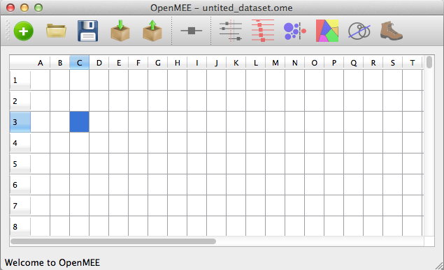
Launch the program by clicking on LaunchOpenMEE.exe in the case of Windows or, on Mac, the OpenMEE app. This will open the main spreadsheet. Sometimes this can take a few seconds.
You will enter and interact with your data via this spreadsheet. From this spreadsheet you can enter your data in the following ways:
Entering the data manually by typing it in to the spreadsheet.
Opening a previously saved dataset (.ome) file
Importing a CSV file (with or without column headers)
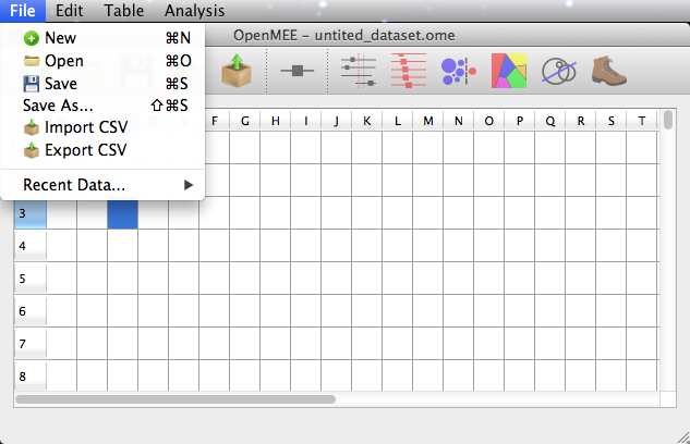
The latter two are accessible via the File menu.
Figure 2. The File menu
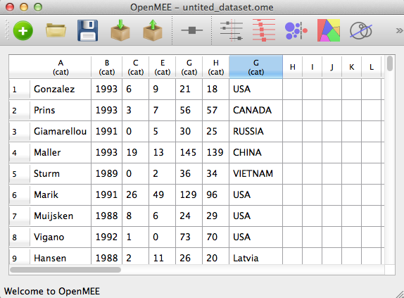
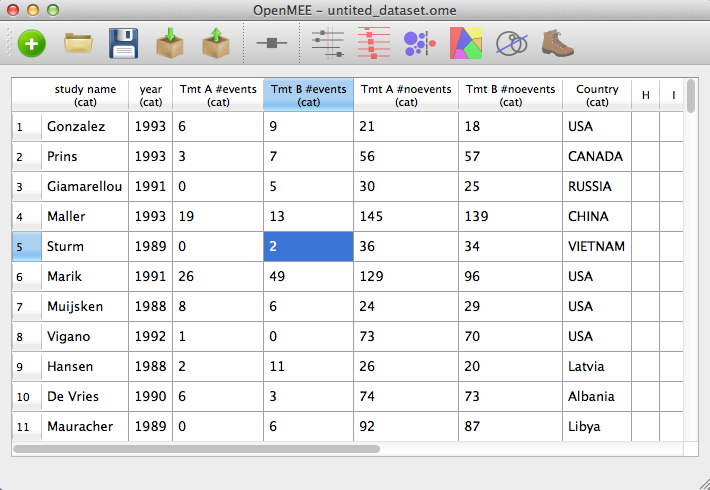
The OpenMEE spreadsheet is very flexible. It has an unlimited number of rows and columns. The spreadsheets starts off with a fixed (large) size. As your data approaches the limits, the spreadsheet automatically resizes itself to accomodate more data. You also don't have to worry about formatting your data beforehand. Simply enter your data in whatever format you have it. For example, After typing in some two-by-two contingency table data we see the screen below.
Figure 3. Main screen after typing in data
Along the top of the spreadsheet we see columns labelled 'A', 'B', 'C', etc., along with '(cat)'. When you enter data into a new column, OpenMEE assumes by default that said column is a new categorical variable and assigns it a default name. When you are done typing in new data, you have to tell OpenMEE what kind of data type each column contains (e.g., continuous). You also must mark one column as the study labels column.
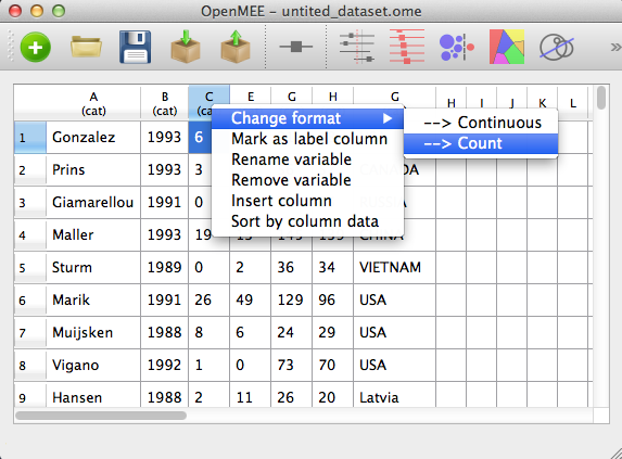
In addition to telling OpenMEE the types of each column, you may also assign your own custom labels (names) to each column. All this is done by right-clicking on column headers and choosing the desired option as shown below:
Figure 4. Context menu, accessible by right-click.
You can rename columns by clicking on the 'rename variable' option of the context menu.
Figure 5. After renaming columns.
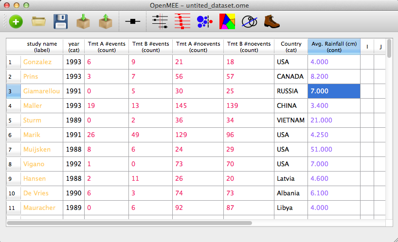
We now have to tell OpenMEE what type of data these columns contain. Again, this is done by right-clicking and selecting a target format from the Change format submenu as shown in Figure 4. Since this is two-by-two data, the four numerical columns are 'counts' while 'Country' and 'Year' are categorical variables, and 'study_name' is the variable we will mark as containing study labels (by selecting 'Mark as label column' from the context menu). Finally out of pedagogical necesssity, let's add a continuous column after country called 'Avg. Rainfall (cm)'. After assigning all these formats, we see
Figure 6. After Setting Variable Formats
Note that for each variable format has its own color scheme as reminder when you're working with the spreadsheet. If you can't stand the default color scheme you can change it by clicking on the Table menu and then Table Preferences:
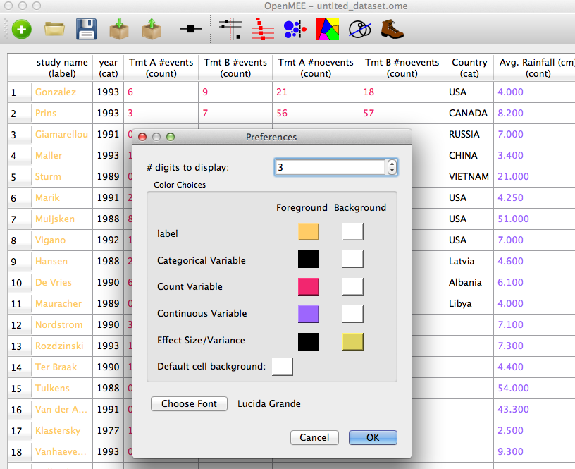
Figure 7. Preferences
Here, you can change the color schemes of the variables as well as the font used on the spreadsheet as well as the number of digits displayed for continuous variables.
Before we can run an analysis, we need effect sizes and associated variances. These can be input in one of two ways:
Entering an effect size and variance manually (i.e., not entering 'raw data')
Calculating an Effect Size from the raw data
We will consider each option in turn
Entering an effect size and variance manually
To do this, simply create two new continuous variables using the method described above. Let's call them "my effect size" and "my variance". Now we need to tell OpenMEE that these are effects. Right-click on the header for "my effect size" and choose Change format → Trans. Effect. Likewise, choose 'Change Format → Trans. Var' for "my variance" as shown in the Figure below.
Figure 8. Changing continuous variance to transformed-scale effect
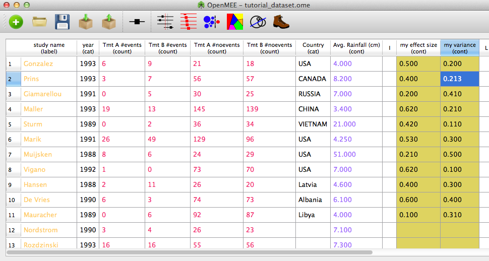
We will then see the screen below
Figure 9. After setting effect size format.
Here we need to discuss the issue of 'transformed' scale vs. 'raw' scale. To perform a meta-analysis, we need an effect size and a measure of dispersion for each study. For example, if our metric is the odds ratio, we need the effect size on the transformed (log) scale because confidence intervals for odds ratios are generally not symmetric in the raw (untransformed) scale. Fortunately, OpenMEE can transform an effect size and confidence interval (or effect size and variance) from one scale another.
Calculating an effect size from raw data
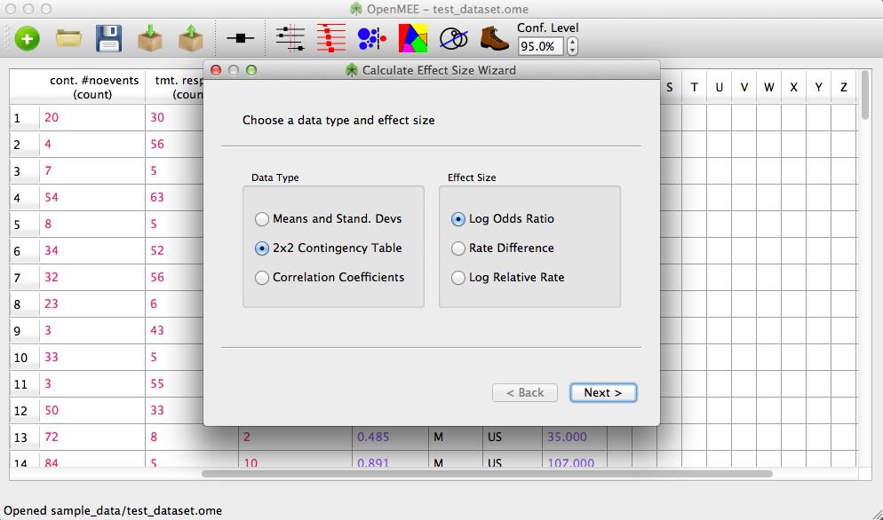
Figure 10. Calculate Effect Size Wizard
To calculate an effect size from raw data, click the 'Calculate Effect Size' button on the toolbar, or select 'Calculate Effect Size' from the analysis menu. This will show the wizard in Figure 10. First, you have to select a data type and a metric.
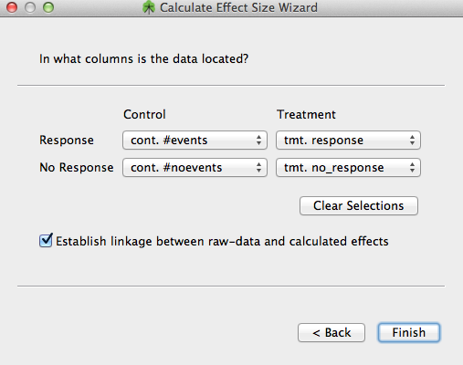
Figure 11. Data location selection
Next tell OpenMEE the locations of the necessary variables as show in Figure 11. You will be given the option to link the raw data columns to the resulting effect size columns (selected by default). This makes it so that when you change a value in the raw data, the effect column will update automagically.
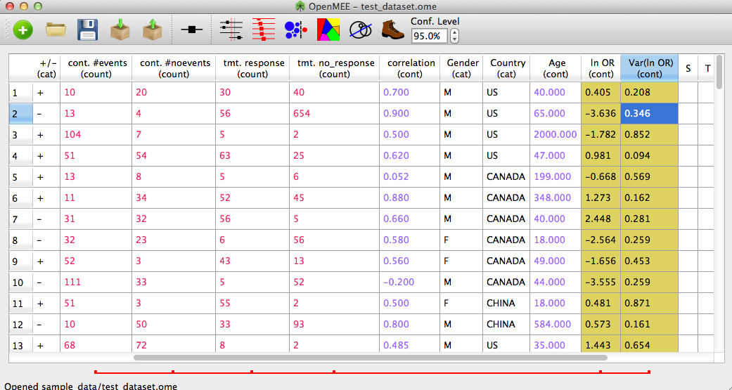
Figure 12. Calculated effect size.
In Figure 12, we see the calculated effect size and variance in the 'transformed' (natural log) scale. Also, note that on the bottom of the window we see a red bar. This provides a visual cue that the four raw data columns cont. #events, #cont #noevents, etc are 'linked' to the effect and variance columns.
Figure 13. Transformed Effect Size Result
In Figure 13, we see the result of transforming the effect size. Three new columns have been added containing the 'raw scale' effect size and upper and lower confidence bounds given the current confidence level shown in the toolbar. Changing the confidence level in the toolbar will cause the confidence interval to be recalculated.
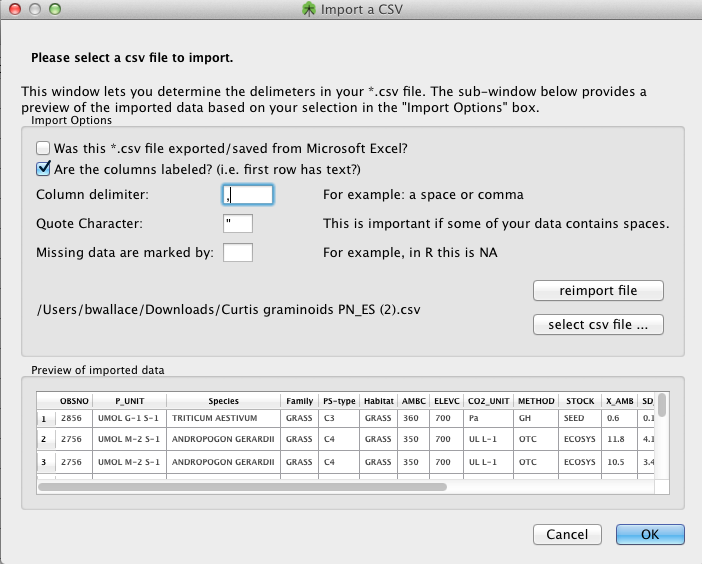
In some cases, one may already have data that one would like to import for analysis. OpenMEE supports importing comma (and otherwise) delimited data. To achieve this, select Import CSV from the File menu. You will be prompted with a screen asking for details about your file format and its location, like so:
Once a file to be imported has been selected, a preview of how it will be read is shown in the small window. Note the field for special strings that denote missing data (you may want to use "NA" here, if importing from R).
Exporting data follows the reverse of the above (select Export CSV rather than Import CSV). Note that all calculated effects and variances will also be exported. Most programs, including Excel (for example), can read CSV's.
All analyses are performed similiarly. You can choose to perform an analysis by clicking its icon in the toolbar or by selecting it from the Analysis menu. More exotic analyses (such as 'bootstrapped' meta regression, meta-regression-based conditional means and boostrapped meta regression-based conditional means) are only accessible from the menu bar.
Here we describe the pages one sees on the wizards for each analysis (this is similar for all analyses).
Here we refer to analyses that look to estimate a 'grand mean', i.e., with no covariates. The pages you will see are as follows.
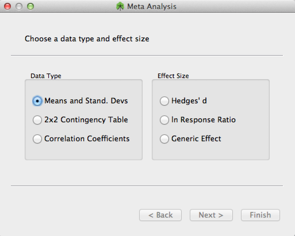
Data Type and Metric
Here you will need to select the data type and effect size. Note that for the latter, you can elect a 'generic effect' if you need.
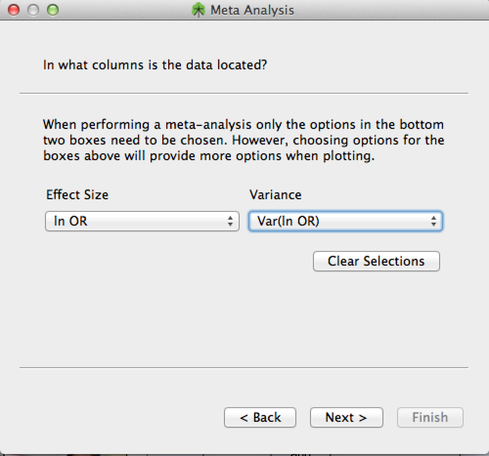
Data Location
Now you will need to select your effect size and variance columns. Here, for example, we have selected ln OR and the variance thereof. In general, the effect size and variance combo boxes will allow you to select any columns that you have designated as effect sizes and variances, respectively.
Refine studies/categories/exclude studies with specific missing data
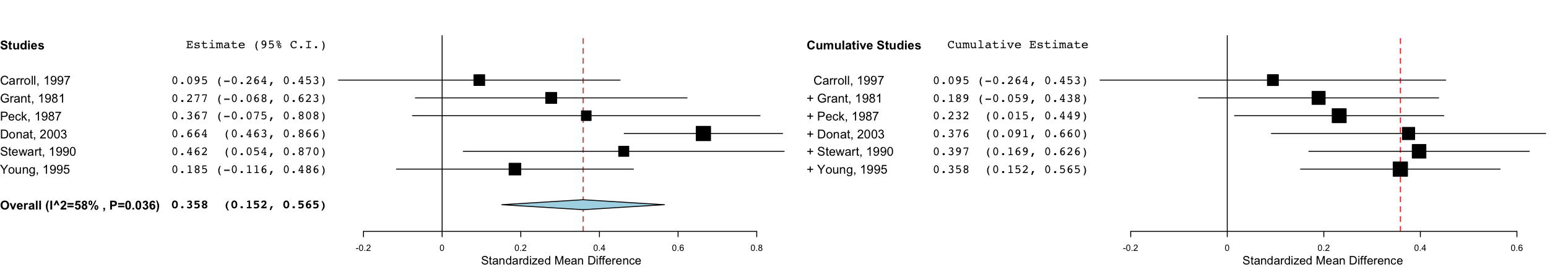
Cumulative meta-analysis is a meta-analytic approach in which studies are added one at a time, and the change in the cumulative effect size is observed. To perform a cumulative meta-analysis in OpenMEE, simply select Cumulative Meta-Analysis from the Analysis menu. We show a sample forest plot generated from a cumulative meta-analysis below. The left-hand side displays the usual study estimates and confidence intervals; the right hand side shows the effect on the overall (summary) estimate as studies are included in the meta-analysis.
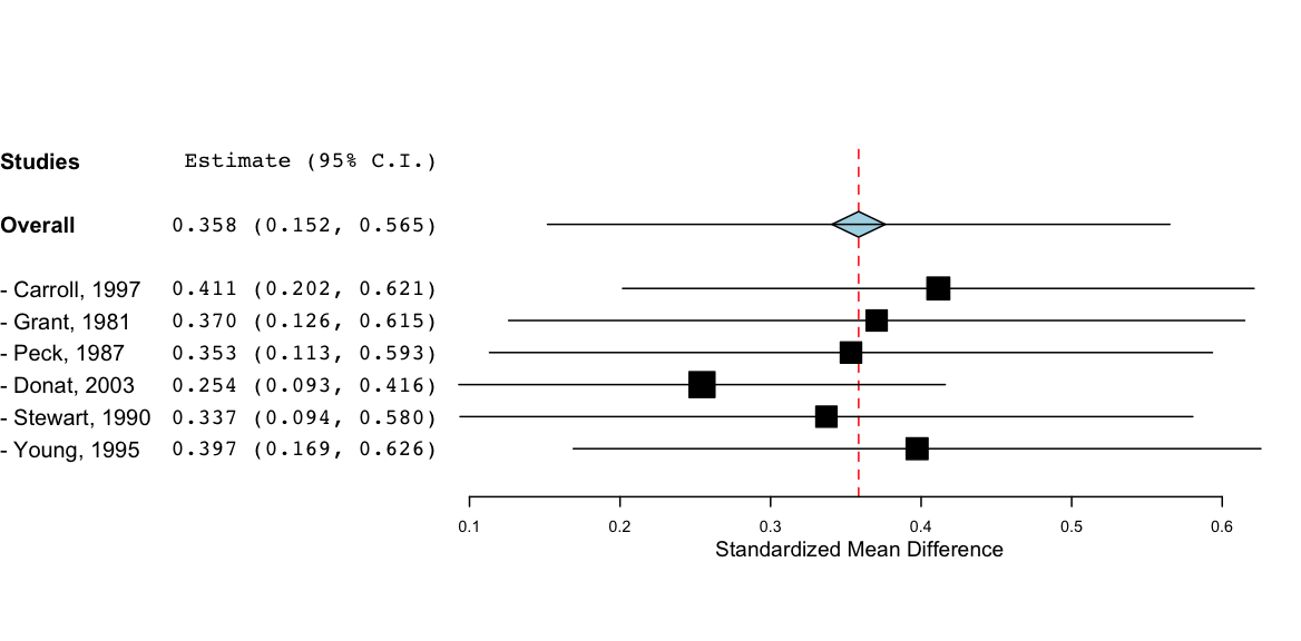
Leave-one-out meta-analysis is conceptually similar to cumulative meta-analysis, except that instead of adding studies one at a time, one holds each study out in turn. This is an exploratory exercise that may highlight influential studies (summary estimates that leave influential studies out will differ substantially than those that include them). An example of output from a leave-one-out analysis is shown below.
Note that the options for Cumulative Meta Analaysis and Leave-One-Out meta analysis are the same as for standard meta-analysis (as described above).
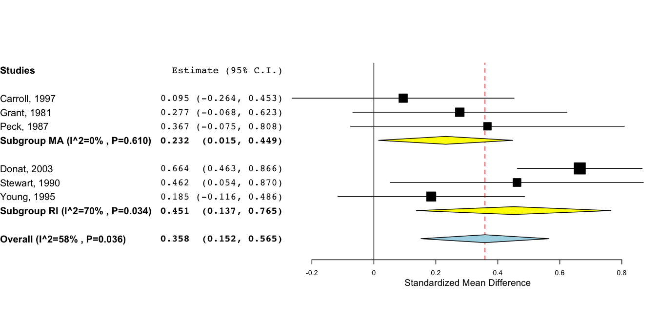
In subgroup meta-analysis, one partitions studies into disjoint groups (e.g., studies conducted in China versus all others) and runs separate meta-analyses over these groups of studies. This is an exploratory exercise that may highlight differences between groups. The options for subgroup meta analysis are the same as for standard meta analysis except for a categorical variable must be selected. For example, if the selected variable is state, then subgroup analyses will be run on studies from each observed state. In the example shown below, this includes Massachusetts (MA) and Rhode Island (RI).
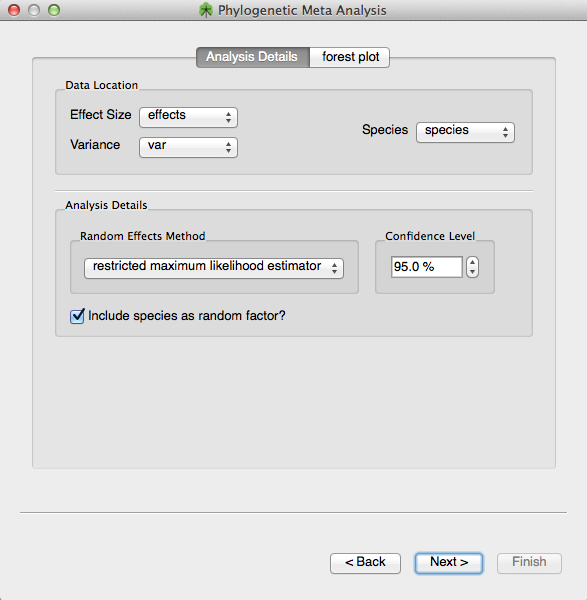
OpenMEE can also do phylogenetic meta-analysis. What this means in practice is that OpenMEE can use a phylogenetic tree to augment the variance for each study based on a SPECIES covariate. As shown below, the phylogenetics meta-analysis wizard requires you to select a column representing the species.
Choose effect size and variance and also a species column
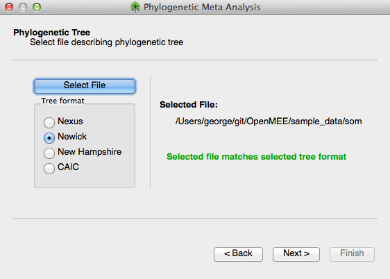
You then have to select a phylogenetic tree file. The file must contain species that match those in the previously selected SPECIES column exactly. The file can be in Nexus, Newick, New Hampshire, or CAIC format.
Choose a phylogenetic tree file
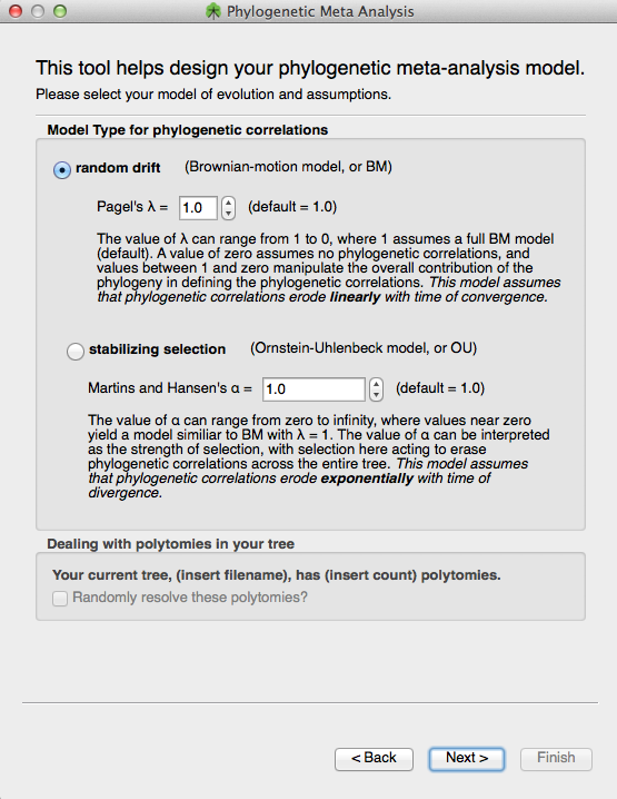
Finally, you can give details about the phylogenetic model type, specifying a Brownian-Motion or Ornstein-Uhlenbeck model.
Meta-regression allows one to explore the relationship between covariates and study outcomes. OpenMEE supports mulitple regression and both continuous and categorical predictors (covariates).
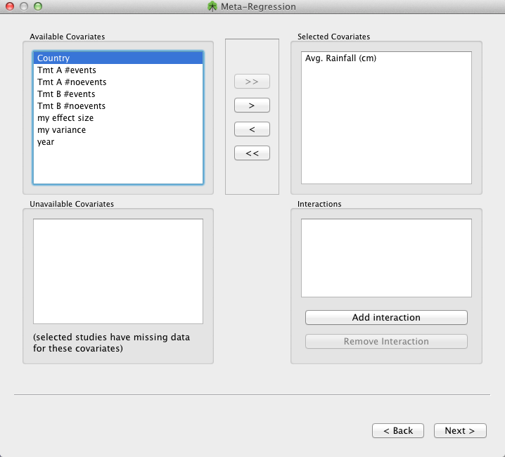
On the 'Select covariates for regression page', select the covariates for regression. On this same page, one can choose whether you want to use a random or fixed effects model and the confidence level to use in the analysis. An example of this is shown below; here we have selected "Avg. Rainfall" to be included in the regression.
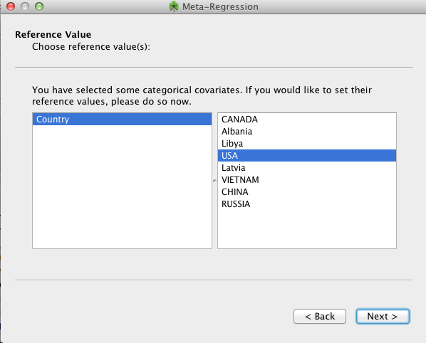
For any categorical covariates that have been selected to be included in the meta-regression, one needs to specify the value that will serve as its reference value (i.e., the intercept). We show an example below where the covariate is Country and the reference value has been specified as USA.
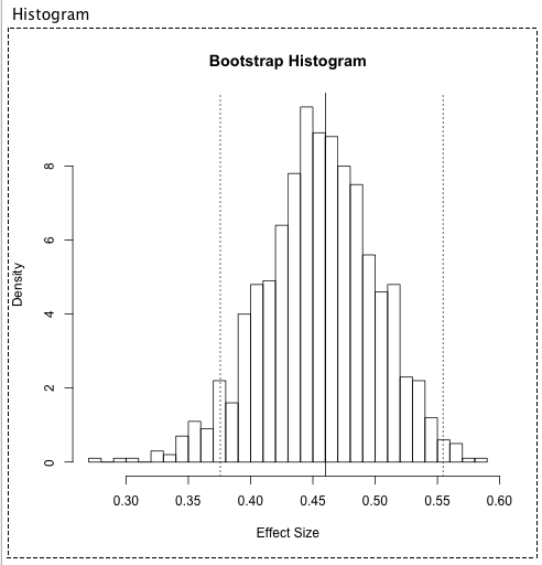
We note that one can also assess the variance of regression coefficient estimates via bootstrapping (see below). To do so, simply select 'bootstrap' rather 'parametric' under 'Type of Analysis' when specifying meta-regression options. We show an example of bootstrap output for the rainfall predictor below.
OpenMEE can compare two regression-models in terms of model-fit statistics and a likelihood ratio test. This is a strategy to assess the informativeness of a given (set of) predictors.
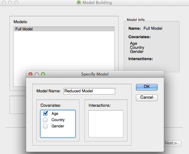
The process to do this model building comparison is very similiar to that of meta-regression. The only differences are that the covariates you select on the covariate select screen will be the covariates used to construct the Full model. You then select a subset of these covariates/interactions to use for the reduced model as shown in the figure.
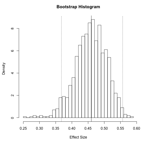
Bootstrapping is a non-parametric approach for assessing the variance of a parameter estimate. OpenMEE allows for bootstrapped estimates both for meta-regressions and standard meta-analysis.
In general, the options for boostrapped meta-analysis are the same as those for standard meta-analysis, with the addition that one needs to provide bootstrap-specific parameter values. These include the number of bootstrap replicates to perform, for example. We show sample output from a boostrapped meta-analysis below.
When running bootstrap operations in OpenMEE, the program tries to generate results using the selected number of bootstrap replicates. We note that depending on the dataset and the meta-anaytic (pooling) model being used, a meta-analysis of a specific sample of the dataset may fail. OpenMEE hands this in a straight-forward way: if one particular replicate attempt fails, another is tried, and so on until 5 times the selected of bootstrap replicates have been attempted, at which point an error message is returned.
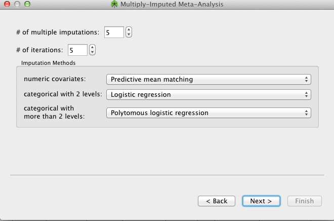
Sometimes data elements are missing from studies. OpenMEE supports basic imputation of covariates for meta-regression. To use this, select Multiple Imputations Meta-Regression form the Analysis drop-down menu. You will be prompted with the following screen
These parameters specify the imputation method to use and the number of multiple imputations to perform. Providing the methodological details of the imputation is beyond the scope of this document, but we refer the interested reader to the R MICE documentation for more details: we use this package 'under the hood' to perform the imputation.
OpenMEE offers various tools to help you visually explore your data including scatterplots and histograms.
Scatterplots
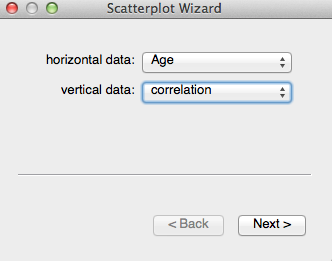
Scatterplots are useful for seeing relationships between two quantitative variables. You can make a scatter plot in OpenMEE by choosing 'Scatterplot' from the 'Data Exploration' menu.
Choosing Scatterplot Data Scatterplot parameters
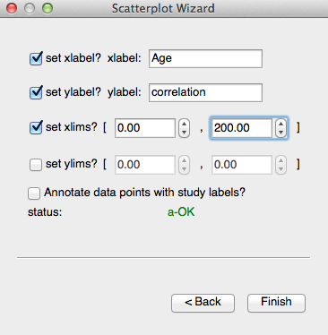
You are presented with a wizard which will allow to choose the source of your data for each axis, then choose custom axis labels and limits. You can also choose to annotate each data point with the study that the point comes from.
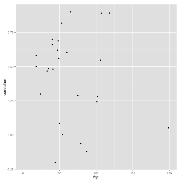
Here is a scatterplot obtained by comparing Age with Correlation:
Example Scatterplot
Histograms
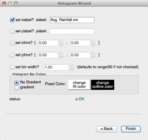
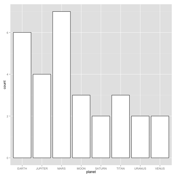
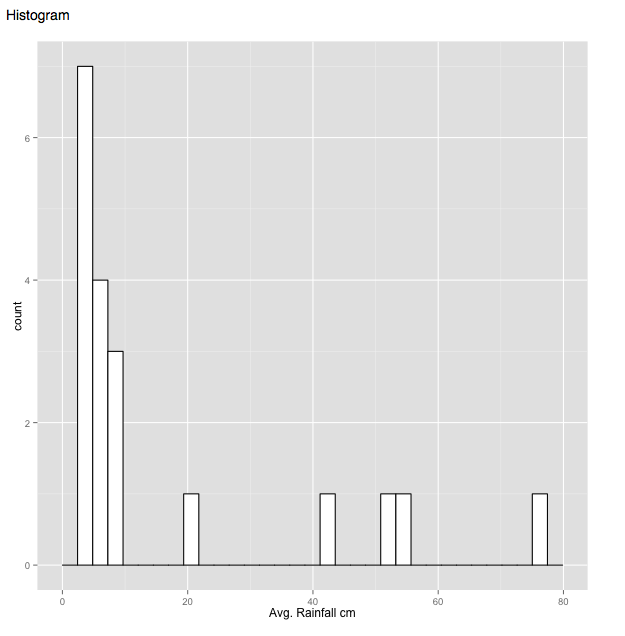
Histograms are a way to look at data, one variable at a time. For quantitative data, the values are 'binned' and then counted. For categorical variables, the count of each level corresponds to the height of each bar. In the figures below, we see the histogram details screen and also an example of a historgram of quantitative data (rainfall) and categorical data (planet),
Histogram details Histrogram of planets (categorical variable) Histogram of rainfall (quantitative variable)
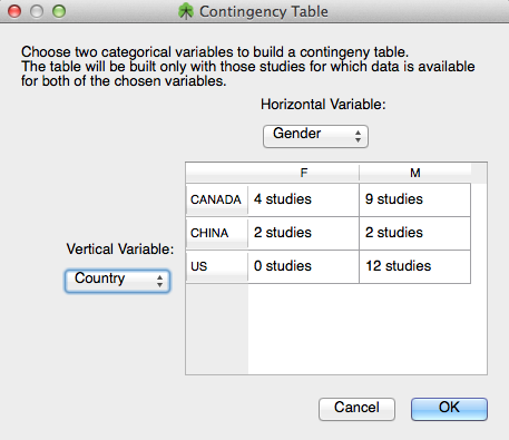
Contingency Table
The contingency table can be used to count the # of studies at each pair of levels between two categorical covariates of interest. This can be useful, for example, when making sure you have enough data for a meta-regression. A contingency table comparing Gender and planet is show below:
Figure 7. Contingency Table
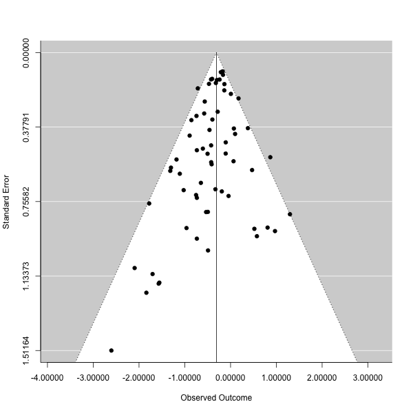
OpenMEE includes the standard tools for publication bias diagnostics, including funnel plots. These can be generated by selecting the Funnel Plot option under the Publication Bias sub-menu of Data Exploration. Example output is shown below. We caution users to interpret these with care, and to read this criticism of funnel plots.
Under the same Publication Bias sub-menu, one can find an option to calculate fail-safe N
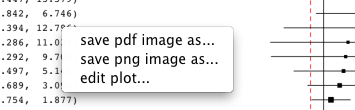
One may wish to export the results from analyses for input into different programs (e.g., Microsoft Word). OpenMEE facilitates this in a few different ways. For images (e.g., forest plots), perhaps the easiest thing to do is to right-click and select "save png image as..." from the context menu, as shown below.
Using this approach, one may save the image to wherever is convienent and then incorporate it into documents. Note that we also support saving as PDF; this is in many cases preferable to PNG, because PDF's are vector graphics. These are to be preferred for publications.
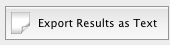
Concerning textual output, such as tables, one can similarly use the contextual menu that is accessible via right-click. Specifically, this involves right-clicking on the textbox of interest and choosing "select all", and then right clicking again and selecting "copy". Results can then be pasted into, e.g., a Word document. Alternatively, one may instead use the "Export Results as Text Button" button:
This will save all displayed textual output to a file of the user's choice.
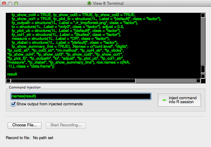
OpenMEE relies on R to perform its analyses. The casual user need not ever be aware of this in the course of his analyses. However, If desired you can see the commands being sent to R in real-time and even interact with the R console. You can also log the R commands to a text file. All this can be done by selecting 'R output viewer' in from the 'Through the looking glass menu'. Then, as you interact with program, the commands being sent to R will appear in the window. This can be useful to automate reproduction of results.
Figure 1. R console
You can interact with objects in the R workspace by typing commands in to the 'Command Injection' area of the 'R output viewer' window and then pressing enter or pushing the 'Inject Command' button.
First of all, did you extract the program to somewhere where you have write privileges as described in the 'Getting Started' section of this document? If you insist on putting the program in a strange place where you don't have write privileges, you can run it if you right-click it, and choose "Run as administrator" under windows or launch it from the command line in Mac via sudo. Don't do this though. Just run the program from where we say to! The desktop is a fine place.
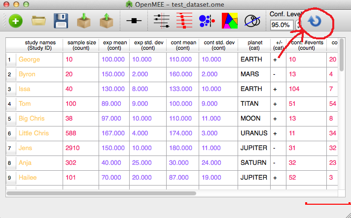
I opened my dataset that I made in a previous build of OpenMEE and 'weird' things are happening when I try to run an analysis.
This can happen if we updated the underlying format of the files we use to store data about datasets. If this happens, you can fix it most of the time by clicking the swirly blue arrow on the upper right of the toolbar and then saving(see the figure). This should update your dataset to be fully compatible with your new version of OpenMEE.
Reset dataset parameters
I'm getting 'Crazy R Errors' when I try to run a meta-analysis or meta-regression
First of all, are your effect sizes reasonable? Not infinity? Make sure you're not dividing by zero somewhere. For meta-regression, are you trying to run it with too many covariates/interactions? This can cause problems with rank of matrices when the number of studies is not large compared to the number of covariates / levels in a categorical covariate.
I don't like the colors in the spreadsheet
Sorry you don't like our taste in colors, you can change them if you like from the Preferences menu.